Getting data into a graph

Now that we know Raphtory is installed and running, let’s look at the different ways to get some real data into a graph.

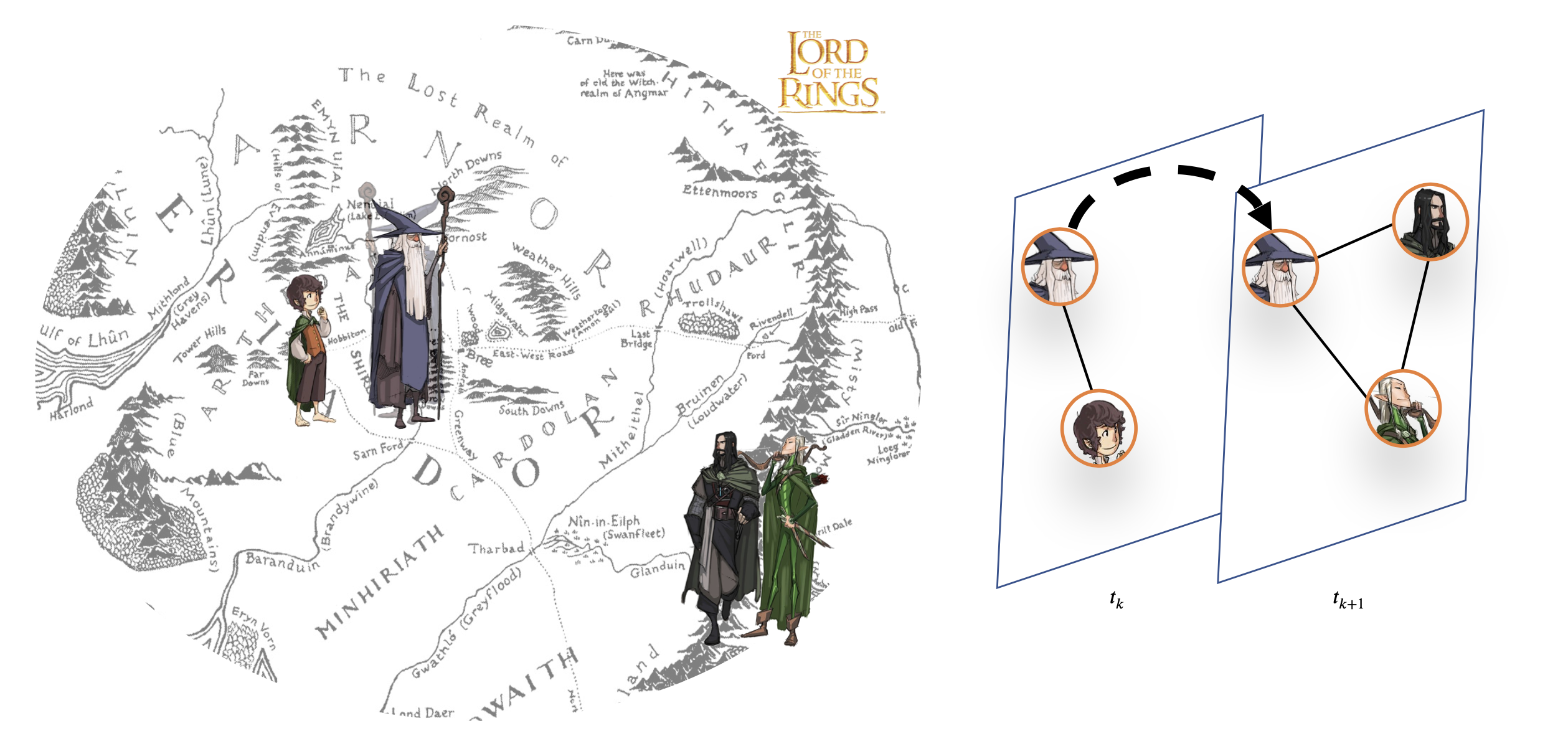
For this first set of tutorials we are going to be building graphs from a Lord of the Rings dataset, looking at when characters interact throughout the trilogy 🧝🏻‍♀️🧙🏻‍♂️💍.

As with the quick start install guide, this and all following python pages are built as iPython notebooks. If you want to follow along on your own machine, click the open on github link in the top right of this page.

Let’s have a look at the example data

The data we are going to use is two csv files which will be pulled from our Github data repository. These are the structure of the graph (lotr.csv) and some metadata about the characters (lotr_properties.csv)

For the structure file each line contains two characters that appeared in the same sentence, along with the sentence number, which we will use as a timestamp. The first line of the file is Gandalf,Elrond,33 which tells us that Gandalf and Elrond appears together in sentence 33.

For the properties file each line gives a characters name, their race and gender. For example Gimli,dwarf,male.

Downloading the csv from Github 💾

The following curl command will download the csv files and save them in the tmp directory on your computer. This will be deleted when you restart your computer, but it’s only a couple of KB in any case.

print("****Downloading Data****")
!curl -o /tmp/lotr.csv https://raw.githubusercontent.com/Raphtory/Data/main/lotr.csv
!curl -o /tmp/lotr_properties.csv https://raw.githubusercontent.com/Raphtory/Data/main/lotr_properties.csv
!curl -o /tmp/lotr.db https://raw.githubusercontent.com/Raphtory/Data/main/lotr.db
print("****LOTR GRAPH STRUCTURE****")
!head -n 3 /tmp/lotr.csv
print("****LOTR GRAPH PROPERTIES****")
!head -n 3 /tmp/lotr_properties.csv

****Downloading Data****
  % Total    % Received % Xferd  Average Speed   Time    Time     Time  Current
                                 Dload  Upload   Total   Spent    Left  Speed
100 52206  100 52206    0     0   154k      0 --:--:-- --:--:-- --:--:--  160k
  % Total    % Received % Xferd  Average Speed   Time    Time     Time  Current
                                 Dload  Upload   Total   Spent    Left  Speed
100   686  100   686    0     0   2906      0 --:--:-- --:--:-- --:--:--  2995
  % Total    % Received % Xferd  Average Speed   Time    Time     Time  Current
                                 Dload  Upload   Total   Spent    Left  Speed
100 69632  100 69632    0     0   287k      0 --:--:-- --:--:-- --:--:--  296k
****LOTR GRAPH STRUCTURE****
Gandalf,Elrond,33
Frodo,Bilbo,114
Blanco,Marcho,146
****LOTR GRAPH PROPERTIES****
Aragorn,men,male
Gandalf,ainur,male
Goldberry,ainur,female

Setting up our imports and Raphtory

Now that we have our data we can sort out our imports and create the Raphtory Graph which we will use to build our graphs.

The imports are for parsing CSV files, accessing pandas dataframes, and bringing in all the Raphtory classes we will use in the tutorial.

The filenames are pointing at the data we just downloaded. If you change the download location above, make sure to change them here as well.

import csv
import pandas as pd
from raphtory import Graph

structure_file = "/tmp/lotr.csv"
properties_file = "/tmp/lotr_properties.csv"
graph = Graph(1)

Adding data directly into the Graph

The simplest way to add data into a graph is to directly call the add_vertex and add_edge functions, which we saw in the quick start guide. These have required arguments defining the time the addition occurred and an identifier for the entity being updated. These functions, however, have several optional arguments allowing us to add properties and within this, types, on top of the base structure.

Function	Required Arguments	Optional Arguments
add_vertex	timestamp,vertex_id	properties
add_edge	timestamp,src_id,dst_id	properties

Lets take a look at this with our example data. In the below code we are opening The Lord of The Rings structural data via the csv reader and looping through each line.

To insert the data we:

• Extract the two characters names, referring to them as the source_node and destination_node.

• Extract the sentence number, referring to is as timestamp. This is then cast to an int as epoch timestamps in Raphtory must be a number.

• Call add_vertex for both nodes, setting their type to Character.

• Create an edge between them via add_edge and label this a Co-occurence.

with open(structure_file, 'r') as csvfile:
    datareader = csv.reader(csvfile)
    for row in datareader:

        source_node = row[0]
        destination_node = row[1]
        timestamp = int(row[2])

        graph.add_vertex(timestamp, source_node, {"vertex_type": "Character"})
        graph.add_vertex(timestamp, destination_node, {"vertex_type": "Character"})
        graph.add_edge(timestamp, source_node, destination_node, {"edge_type": "Character_Co-occurence"})

Let’s see if the data has ingested

To do this, much like the quick start, we can run a query on our graph. As Raphtory allows us to explore the network’s history, lets add a bit of this in as well.

Below we check the data contained in the graph by running the earliest_time(), latest_time(), and len the vertices and edges.

print("Earliest time: %i" % graph.earliest_time())
print("Latest time: %i" % graph.latest_time())

print("Number of vertices: %i" % len(graph.vertices()))
print("Number of edges: %i" % len(graph.edges()))

Earliest time: 33
Latest time: 32674
Number of vertices: 139
Number of edges: 701

We can also access a specific vertex, such as Gandalf, and see his degree at different points in time using the at() function.

In the first call, we get the entire graph at time 1000, and then check the degree of gandalf.

In the second call, we get the vertex gandalf, get their instance at time 10,000 and the degree.

print("Gandalf's degree at 1000: %i" % graph.at(1000).vertex("Gandalf").degree())

print("Gandalf's degree at 10,000: %i" % graph.vertex("Gandalf").at(10000).degree())

Gandalf's degree at 1000: 4
Gandalf's degree at 10,000: 26

Updating graphs, merging datasets and adding properties

One cool thing about Raphtory is that we can freely insert new information at any point in time and it will be automatically inserted in chronological order. This makes it really easy to merge datasets or ingest out of order data.

A property on a vertex or edge can be either static or non-static.

• Static properties, do not change and are fixed throughout the life of the graph, e.g. the name property.

• Non-static properties can change over time, e.g. balance of a bank account.

All property objects require the user to specify a name and value.

To explore this and to add some properties to our graph, lets load our second dataset!

Below we are opening our property file the same way as the structure file. This data does not have a time element, so we can add the properties as static properties. This means they will be available at evert point in time and the values will stay the same.

Now it’s worthwhile noting that we aren’t calling a function called update_vertex or something similar, even though we know the vertex exists. This is because everything is considered an addition into the history and Raphtory sorts all the ordering internally!

with open(properties_file, 'r') as csvfile:
    datareader = csv.reader(csvfile)
    for row in datareader:
        graph.add_vertex_properties(row[0], {"race": row[1],"gender": row[2]})

Using our properties as part of a query

To quickly see if our new properties are included in the graph we can write a new query! Lets have a look at the dwarves who have the most interactions.

To start we can create a function which for each vertex and check the size of exploded edges. This takes each edge and measures how many times it was updated. E.g. if Gimli and Balin met four times, in the graph they have one edge between them. But if we explode this edge, we can see each time they met.

We can iterate through each vertex and filter by the race property and remove anyone who isn’t a dwarf.

Finally, we can sort the data into a dataframe to see Gimli has by far the most!

result = []
# This returns an iterator, so we should store the value to avoid a deadlock
vertices = list(graph.vertices())

for vertex in vertices:
    if vertex.property("race") == "dwarf":
        interactions = sum([len(e.explode()) for e in vertex.edges()])
        latest = vertex.latest_time()
        result.append({"timestamp": latest, "name": vertex.name(), "interactions": interactions })

pd.DataFrame(result).sort_values(by="interactions",ascending=False)

	timestamp	name	interactions
3	31247	Gimli	185
1	31129	Glóin	31
2	10938	Balin	14
0	9605	Thorin	5